GAN
Authors: Daniel Gao, Edward Qin
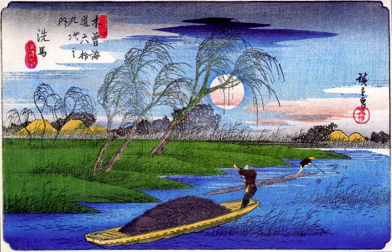 Sample of Japanese Art from the training dataset
Introduction
Our goal for this project was to generate new visual art in the style of Japansese art from the Muromachi period (1392-1573) all the way to the Shōwa period (1926-1989). We used a Generative Adversarial Network (GAN), which is composed of a generative and discriminative network. The dataset we used is the Japanese Art directory from the WikiArt Art Movements/Styles dataset on Kaggle.
Check out our model on Google Colab and our video demo!
GAN Model
A GAN is a generative adversarial network, which is composed of a generator and discriminator model. The discriminator attempts to determine if input images are part of the training dataset (labeled 1) versus if they are from the generated fake images (labeled 0). The generator attempts to generate images to fool the discriminator into thinking they are real.
In this project, we use a DCGAN, a deep convolutional GAN, which uses convolutional and convolutional-transpose layers in the discriminator and generator respectively.
If $x$ represents the input image data, then $D(x)$ represents the probability that the discriminator determines that $x$ came from the training dataset.
Now suppose we have a latent space vector $z$ composed of random values such that when fed to the generator, $G(z)$ maps $z$ to a data space representing an image. The goal of the generator is to estimate the distribution $p_{data}$ that generates the real images from the training data. Formalized, this is when $D(G(z)) = D(x)$, meaning the discriminator cannot discriminate between real and generate images.
Likewise, the distribution of the generated images $p_g$ is the same as the distribution of the input latent space vector $p_z$. As such, the loss function of the GAN is as follows:
\[\min_G\max_DV(D, G) = \mathbb{E}_{x \sim p_{data}(x)}[logD(x)] + \mathbb{E}_{z \sim p_{z}(z)}[log(1-D(G(z)))]\]We can see that this loss function is similar to the PyTorch BCELoss function which we use in our training.
Version 1
For the first version of our model, we based the architecture on previous work, the PyTorch DCGAN tutorial model.
The input to the generator is $z$, a latent space vector of length 100. In each of the 5 convolutional-transpose layers, we upsample the input by a factor of $2 \times 2$. After each convolutional-transpose before the final convolutional-transpose, we also apply a batch normalization followed by a ReLU activation. On the last convolutional-transpose layer, we do a final $\tanh$ activation function on the $3\times64\times64$ image.
The discriminator architecture is like the inverse of the generator, with input image of size $3 \times 64 \times 64$. We have 5 convolutional layers that each downsample by a factor of $2 \times 2$. We apply batch normalization on layers other than the first and last layer, and all layers other than the last layer use the Leaky ReLU activation function. In the final layer, we apply the sigmoid function to determine the probability that the image is real, $D(x)$.
To train our model, we first resized the 2235 images of our dataset to $64 \times 64$ images. We then used a batch size of 128, learning rate of 0.0005, the Adam optimizer with $\beta_1$ coefficient 0.5 (instead of 0.9 in the tutorial), and 300 epochs.
Below, we provide the plot of the discriminator and generator loss over iterations, as well as the change in the generated images over time.
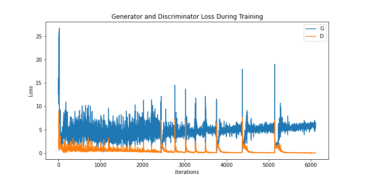
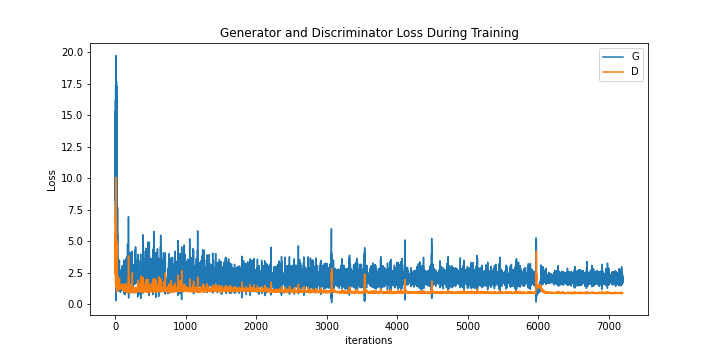
Version 1 Discriminator and Generator Loss
Version 1 Generated Images
From the plot of the losses, we observe that the the discriminator and generator loss start to diverge after 2000 iterations. There is also unexplained spiking for both the discriminator and generator loss after 2500 iterations. However, from the generated images, we notice that the generator struggles to create definitive, structural objects. Some generated images seem to depict landscapes like mountains and bodies of water well, but there are no clear faces on images that seem to generate people.
Version 2
We noticed that in Version 1, our loss function was diverging. This suggested that our discriminator was becoming too accurate too quickly. Thus, we attempted to slow the rate of change in discriminator loss. We took a new approach by applying label smoothing, which changed the labels from 0 and 1 to ranges $[0, 0.3]$ and $[0.7, 1]$, as well as changing the generator’s activation functions from ReLU to Leaky ReLU. These changes were based on tips from this github page.
The image size, batch size, learning rate, and optimizer we used were the same as that of version 1. However, we stopped training after 100 epochs.
Below, we again provide the plot of the discriminator and generator loss over iterations, as well as the change in the generated images over time.
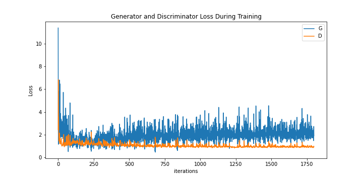
Version 2 Discriminator and Generator Loss
Version 2 Generated Images
From the loss plot, we observe that the discriminator and generator loss begin to diverge after 500 iterations. However, compared to version 1, the overall loss is much lower for both networks. This is likely due to the label smoothing. We also decided to stop training after 100 epochs because we noticed that the images were all following the same blurring and checkerboard pattern.
Version 3
Based on setbacks in Version 2, we decided that we should revert a change made. We reasoned that label smoothing helps the discriminator learn at a lower pace, increasing stability, so we opted to revert the activation function change.
We again used the same image size, batch size, learning rate, and optimizer, but trained for 400 epochs, instead.
As we see below, the plot of the discriminator and generator loss does not diverge as much as the previous versions. We also see that there is more structure in the generated images over time.
Version 3 Discriminator and Generator Loss
Version 3 Generated Images
However, from the loss plot, we see that there is some spiking and divergence after 6000 iterations. We also see that the images sometimes form more convincing and detailed images at an epoch before becoming blurred in a later epoch. In particular, row 4 column 6 of the generated images depicts human figures approximately 2/3 through the training before they vanish into whiteness and form human figures again at near the final epochs.
However, this approach to use label smoothing was ultimately beneficial. We saw less spiking in the loss function, and divergence did not appear until later. In the generated images, we also saw slightly more structure at various points of the training process.
Reflection on setbacks
Throughout the training process, we experienced a few difficulties. First, we saw that the losses were spiking in the version 1 model. We could not determine what exactly caused the spiking, but we recognized that GAN model training is difficult and unstable. We attributed the spiking behavior to mode collapse, where the discriminator was trained too quickly and the generator could only make minor changes before the discriminator learned the generator’s change.
Secondly, we realized that our data was unstructured. The data used in other GAN models has usually been the Celebrity A dataset, where celebrity faces are aligned. However, our images were both unaligned and of different objects. We had both landscapes and people in the art. As such, we noticed that our generator mimicked the Japanese Art style well, but not necessarily the structure of the objects in the image.
Finally, the generated images seemed to converge when we applied both label smoothing and a different activation function in version 2. As depicted in the change of generated images over time, we saw checkerboard-like patterning and blurring in the images, and the loss functions were clearly diverging. As a result, we decided to create version 3 to determine the source of the patterning.
Conclusion
While we believe that the GAN model was successful in generating the art style, we believe that the next steps would be to train for the structure of the images. We could do so by either finding a better dataset or using a different model. Ideally, we would have a larger dataset where images are aligned and do not span art styles in a range of over 5 centuries. We could also use the diffusion model, which while more expensive in training time, is stabler and better at generating images than GANs.
Additionally, we think it would be interesting if, supposing that we successfully train the model, we expanded it to also generate different styles like Romanticism or Baroque art styles in the WikiArt dataset.